한동안 텐서플로우를 놓고 있다가 최근에 회사에서 작업하는 일이 있어 다시 공부하게 되었습니다. 그동안 회귀분석 정도만 필요했기에 딥러닝 알고리즘들을 사용해볼 기회가 적었는데, 이번 기회에 덕분에 손에 잡게 되었네요 :)
이번에 공부해본 예제는 CIFAR 10 입니다.
CIFAR 10?
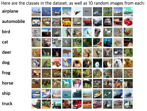
CIFAR 10은 32x32사이즈의 RGB 이미지 데이터셋으로, 10가지의 레이블이 붙어있습니다. 작은 이미지지만, 머신러닝 알고리즘을 통해 10개의 레이블로 예측해보는 연습을 할 수 있습니다.
다만 데이터셋이 확실히 MNIST보다는 무겁기 때문에, 처음 연습하시는 분이라면 먼저 MNIST를 한 뒤에 해보시는 걸 추천드립니다.
(원리는 동일합니다. 다만 RGB 3레이어가 껴있다는 데서 벡터 연산만 약간~ 다를 뿐입니다)
전체적인 특징은 다음과 같습니다.
- VANILLA CNN 알고리즘을 사용합니다. CNN을 응용한 Resnet, Inception 등을 사용하지 않고, 순수히 Convolutional한 뉴럴넷만 사용했습니다.
- TensorBoard를 사용해봤습니다. 텐서보드는 아래 코드로 짠 부분을 그래픽컬하게 표현해주는 도구인데, scalar값을 epoch나 batch에 따라 기록을 저장해서 그래프로 보여줄 수 있습니다. 즉, epoch에 따라 줄어가는 cost, 높아져가는 accuracy 값을 확인할 수 있어요.
- MNIST와 다르게 데이터셋에 다음 batch 항목을 보여주는 기본 함수가 없습니다. 그래서 batch_size만큼 다음 데이터를 가져오는 함수를 만들어놨습니다.
- Train / Test 정확도는 약 70~80% 수준으로 나왔습니다.
- 다음에는 동일한 코드에, Batch Normalization만 추가해서 얼마나 정확도가 올라가는지 한번 비교해볼게요 :)
전체 코드는 아래와 같습니다.
아주 기본적인 코드로, 공부하시는 분들께 조금이나마 도움이 되었으면 좋겠습니다.
1 2 3 4 5 6 7 8 9 10 11 12 13 14 15 16 17 18 19 20 21 22 23 24 25 26 27 28 29 30 31 32 33 34 35 36 37 38 39 40 41 42 43 44 45 46 47 48 49 50 51 52 53 54 55 56 57 58 59 60 61 62 63 64 65 66 67 68 69 70 71 72 73 74 75 76 77 78 79 80 81 82 83 84 85 86 87 88 89 90 91 92 93 94 95 96 97 98 99 100 101 102 103 104 105 106 107 108 109 110 111 112 113 114 115 116 117 118 119 | import tensorflow as tf from tensorflow.keras.datasets.cifar10 import load_data # 추후 모델을 재사용하기 위해 세이브합니다. save_file = './model.ckpt' # CIFAR10 모델을 불러옵니다. (x_train, y_train), (x_test, y_test) = load_data() # 기본 데이터의 Y레이블은 0~9 까지의 값으로 되어 있어서, 이를 one-hot-encoding 형태로 벡터화 해주는 작업 y_train_one_hot = tf.squeeze(tf.one_hot(y_train, 10), axis=1) y_test_one_hot = tf.squeeze(tf.one_hot(y_test, 10), axis=1) # 기본 설정 값들 tf.set_random_seed(777) learning_rate = 0.0001 training_epoch = 15 batch_size = 100 X = tf.placeholder(tf.float32, [None, 32, 32, 3]) Y = tf.placeholder(tf.float32, [None, 10]) # 5개의 CNN 기본 레이어를 거친 뒤, FC 레이어로 바꿔줍니다. W1 = tf.Variable(tf.random_normal([3, 3, 3, 64], stddev = 0.01)) L1 = tf.nn.conv2d(X, W1, strides = [1, 1, 1, 1], padding = 'SAME') b1 = tf.Variable(tf.constant(0.1, shape=[64])) h1 = tf.nn.relu(L1 + b1) p1 = tf.nn.max_pool(h1, ksize = [1, 2, 2, 1], strides = [1, 2, 2, 1], padding = 'SAME') W2 = tf.Variable(tf.random_normal([3, 3, 64, 64], stddev = 0.01)) L2 = tf.nn.conv2d(p1, W2, strides = [1, 1, 1, 1], padding = 'SAME') b2 = tf.Variable(tf.constant(0.1, shape=[64])) h2 = tf.nn.relu(L2 + b2) p2 = tf.nn.max_pool(h1, ksize = [1, 2, 2, 1], strides = [1, 2, 2, 1], padding = 'SAME') W3 = tf.Variable(tf.random_normal([3, 3, 64, 128], stddev = 0.01)) L3 = tf.nn.conv2d(p2, W3, strides = [1, 1, 1, 1], padding = 'SAME') b3 = tf.Variable(tf.constant(0.1, shape=[128])) h3 = tf.nn.relu(L3 + b3) W4 = tf.Variable(tf.random_normal([3, 3, 128, 128], stddev = 0.01)) L4 = tf.nn.conv2d(p3, W4, strides = [1, 1, 1, 1], padding = 'SAME') b4 = tf.Variable(tf.constant(0.1, shape=[128])) h4 = tf.nn.relu(L4 + b4) W5 = tf.Variable(tf.random_normal([3, 3, 128, 128], stddev = 0.01)) L5 = tf.nn.conv2d(p4, W5, strides = [1, 1, 1, 1], padding = 'SAME') b5 = tf.Variable(tf.constant(0.1, shape=[128])) h5 = tf.nn.relu(L5 + b5) # FC 레이어 형태로 최종값을 변경한 뒤, 레이블 값 예측에 사용될 logits를 만듭니다. h5_flat = tf.reshape(h5, [-1, 8*8*128]) W6 = tf.Variable(tf.random_normal([8*8*128, 10], stddev = 0.01)) b6 = tf.Variable(tf.constant(0.1, shape = [10])) logits = tf.matmul(h5_flat, W6) + b6 # cost, optimizer 등 선언. softmax_cross_entropy를 사용했습니다. cost = tf.reduce_mean(tf.nn.softmax_cross_entropy_with_logits_v2(logits = logits, labels = Y)) optimizer = tf.train.AdamOptimizer(learning_rate = learning_rate).minimize(cost) corrent_prediction = tf.equal(tf.argmax(logits, 1), tf.argmax(Y, 1)) accuracy = tf.reduce_mean(tf.cast(correct_prediction, tf.float32)) # TensorBoard에서 cost와 accuracy를 그래프화 해보겠습니다. cost_sum = tf.summary.scalar("cost", cost) accuracy_sum = tf.summary.scalar("accuracy", cost) # batch_size(100개)에 맞게 RAW데이터를 쪼개서 return 해주는 함수입니다. def next_batch_train(num, starting_point): x_train_batch = x_train[starting_point:num+starting_point] y_train_batch = y_train[starting_point:num+starting_point] return x_train_batch, y_train_batch # 학습 시작 with tf.Session() as sess: saver = tf.train.Saver() # Tensorboard에 띄우기 위한 writer 작업. merged = tf.summary.merge_all() writer = tf.summary.FileWriter('./CIFAR10_VANILLA_CNN/train', sess.graph) writer_test = tf.summary.FileWriter('./CIFAR10_VANILLA_CNN/test', sess.graph) sess.run(tf.global_variables_initializer()) with tf.device('/gpu:0'): print('Learning Started') for epoch in range(training_epochs): avg_cost = 0 avg_cost_test = 0 total_batch = int(len(x_train) / batch_size) starting_point = 0 for i in range(total_batch): batch_xs, batch_ys = next_batch_train(batch_size, starting_point) feed_dict = {X: batch_xs, Y: batch_ys.eval()} summary, c, a, _ = sess.run([merged, cost, accuracy, optimizer], feed_dict = feed_dict) avg_cost += c / total_batch starting_point += 100 feed_dict_test = {X: x_test, Y: y_test_one_hot.eval()} summary_test, c_test, a_test = sess.run([merged, cost, accuracy], feed_dict = feed_dict_test) avg_cost_test = c_test print('Epoch:', '%04d' % (epoch + 1), 'Train cost =', '{:.9f}'.format(avg_cost)) print('Epoch:', '%04d' % (epoch + 1), 'Train acc =', '{:.9f}'.format(a)) print('Epoch:', '%04d' % (epoch + 1), 'Test cost =', '{:.9f}'.format(avg_cost_test)) print('Epoch:', '%04d' % (epoch + 1), 'Test cost =', '{:.9f}'.format(a_test)) writer.add_summary(summary, global_step = epoch) writer_test.add_summary(summary_test, global_step = epoch) print('Learning Finished') writer.close() saver.save(sess, save_file) | cs |
'Developer > Machine Learning' 카테고리의 다른 글
| [Tensorflow] 학습 모델 저장하고 불러오는 방법 (Saver, Restore) (1) | 2020.01.13 |
|---|---|
| [Tensorflow] MNIST 데이터셋 CNN 기본 예제 (0) | 2020.01.12 |
| Tensorflow CPU/GPU 목록 확인하기 (0) | 2019.12.30 |
| #7. Tensorflow로 linear regression cost 최소화 구현하기 (124) | 2017.11.26 |
| #6. Linear Regression의 cost 최소화 알고리즘 (583) | 2017.11.25 |

댓글